Inverse Distance to a Power
The Inverse Distance to a Power gridding method is a weighted average interpolator, and can be either an exact or a smoothing interpolator.
With Inverse Distance to a Power, data are weighted during interpolation such that the influence of one point relative to another declines with distance from the grid node. Weighting is assigned to data through the use of a weighting power that controls how the weighting factors drop off as distance from a grid node increases. The greater the weighting power, the less effect points far from the grid node have during interpolation. As the power increases, the grid node value approaches the value of the nearest point. For a smaller power, the weights are more evenly distributed among the neighboring data points.
Normally, Inverse Distance to a Power behaves as an exact interpolator. When calculating a grid node, the weights assigned to the data points are fractions, and the sum of all the weights are equal to 1.0. When a particular observation is coincident with a grid node, the distance between that observation and the grid node is 0.0, and that observation is given a weight of 1.0, while all other observations are given weights of 0.0. Thus, the grid node is assigned the value of the coincident observation. The Smoothing parameter is a mechanism for buffering this behavior. When you assign a non-zero Smoothing parameter, no point is given an overwhelming weight so that no point is given a weighting factor equal to 1.0.
One of the characteristics of Inverse Distance to a Power is the generation of "bull's-eyes surrounding the position of observations within the gridded area. You can assign a smoothing parameter during Inverse Distance to a Power gridding to reduce the bull's-eye effect by smoothing the interpolated grid.
Inverse Distance to a Power is a very fast method for gridding. With less than 500 points, you can use the All Data search type and gridding proceeds rapidly.
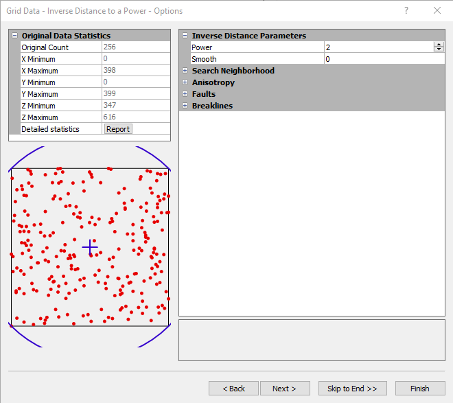
Inverse Distance to a Power Options Dialog
In the Grid Data dialog, specify Inverse Distance to a Power as the Gridding Method and click the Next button to open the Grid Data Inverse Distance to a Power Options dialog.
|
|
|
Specify the parameters to use when gridding with the inverse distance to a power gridding method. |
Power
The weighting Power parameter determines how quickly weights fall off with distance from the grid node. As the power parameter approaches zero, the generated surface approaches a horizontal planar surface through the average of all observations from the data file. As the power parameter increases, the generated surface is a "nearest neighbor" interpolator and the resultant surface becomes polygonal. The polygons represent the nearest observation to the interpolated grid node. Power values between 1.2e-038 and 1.0e+038 are accepted, although powers should usually fall between one and three.
Smooth
The Smooth factor parameter allows you to incorporate an "uncertainty" factor associated with your input data. The larger the smoothing factor parameter, the less overwhelming influence any particular observation has in computing a neighboring grid node.
Search Neighborhood
Specify search rules. For more information about search rules, see Search.
Anisotropy
Set anisotropy settings if needed. For more information about anisotropy options, see Anisotropy.
Breaklines and Faults
Specify a breakline and/or fault. For more information, see Breaklines and Faults. Breaklines and faults are supported when creating a grid surface (XYZ data). Breaklines and faults are not supported when creating a grid volume (XYZC data).
References
Davis, John C. (1986), Statistics and Data Analysis in Geology, John Wiley and Sons, New York. ISBN: 9780471015753
Franke, R. (1982), Scattered Data Interpolation: Test of Some Methods,Mathematics of Computations, v. 33, n. 157, p. 181-200. DOI: 10.2307/2007011