Variogram Grid
Surfer uses a variogram grid as a fundamental internal data representation, in lieu of a pair comparison file. The pair comparison file can be extremely large for moderately sized data sets. For example, 5000 observations create N(N-1)/2 pairs (12,497,500). Each pair requires 16 bytes of information for a pair comparison file, so a 5000-observation pair comparison file would take approximately 191 megabytes of memory to merely hold the pair comparison information. The time to read and search through this large file makes this approach impractical for many Surfer users.
Computational speed and storage are gained by using the variogram grid approach. Once the variogram grid is built, any experimental variogram can be computed instantaneously. This is independent of the number of observations. However, the ability to carry out on-the-fly editing of variograms on a pair-by-pair basis is lost by using the variogram grid approach in Surfer.
Unlike the grids used elsewhere in Surfer, which are rectangular grids, variogram grids are polar grids. Polar grids cannot be viewed in Surfer, and are only used within the context of variogram computation. The first coordinate in a variogram grid is associated with the polar angle, and the second coordinate is associated with the radial distance out from the origin.
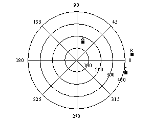
Consider the following variogram grid:
|
|
|
Polar variogram grid for three pairs (A, B, and C) of observation points, showing separation angles and separation distances. |
There are eight angular divisions: {0°, 45°, 90°, 135°, 180°, 225°, 270°, 315°} and four radial divisions: {100, 200, 300, 400}. Thus, there are 32 individual cells in this variogram grid. Users familiar with VarioWin® will notice similarities between Surfer's variogram grid and the "variogram surface" in VarioWin® 2.2. In Surfer, only the upper half of the grid is used. See the General Page for a more detailed explanation.
Consider the following three observation locations: {(50,50), (100, 200), and (500,100)}. There are three observations, so there are 3*(3-1)/2 = 3 pairs. The pairs are:
A (50,50), (100,200)
B (50,50), (500,100)
C (100,200), (500,100)
Each pair is placed in a particular cell of the variogram grid based upon the separation distance and separation angle between the two observation locations.
The separation distance is:
|
|
The separation angle is:
|
|
Using the above equations, the separation angle for the first pair of observations {(50,50), (100,200)} is 71.57 degrees and the separation distance is 158.11. This pair is placed in the cell bounded by the 100 circle on the inside, the 200 circle on the outside, the 45° line in the clockwise direction, and the 90° line in the counterclockwise direction. The location of this pair in the variogram grid is shown on the previous page as point A.
|
Pair |
Separation Angle |
Separation Distance |
|
A |
71.57 |
158.11 |
|
B |
6.34 |
452.77 |
|
C |
-14.04 |
412.31 |
|
The separation angle and separation distance for each pair are calculated using the previous equations. |
||
Since the separation distance of pairs B and C are greater than the radius of the largest circle (400), these pairs fall outside of the variogram grid. Pairs B and C are not included in the variogram grid and therefore, not included in the variogram. Using the above equations, every pair is placed into one of the variogram grid cells or it is discarded if the separation distance is too large.
For a large data set there could be millions of pairs (or more) and the associated pair comparison file would be very large. On the other hand, with the variogram grid in the example above there are only 32 grid cells regardless of the number of pairs contained in a particular grid cell. Herein lies the computational saving of the variogram grid approach. It is not necessary that every pair is stored in a variogram grid cell; each variogram grid cell stores only a small set of summary statistics which represent all of the pairs contained within that cell.

