Grid Volume Report
When Grids | Calculate | Volume computations are executed, the resulting quantitative metrics are compiled and shown within the structural Grid Volume Report window.
The operational breakdowns documented within the report database include the following structural sections:
Upper Surface and Lower Surface
These sections preserve an audit trail of the explicit parameters, grid file structures, or constant Z levels that bound the top and bottom limits of the geometric solid.
Polygon Boundary Log
The Polygon Boundary section displays critical tracking parameters whenever calculation boundaries are applied. The File Name field logs the direct operating system path for the base vector file. The Number of Polygons metric updates to count total boundaries parsed, and the Volume state logs whether interpolation was isolated inside or outside the vertices.
Quantitative Breakdown of Volumetric Metrics
The report separates calculations into discrete structural blocks to help users track total volumetric mass changes:
-
Positive Volume (Cut): The definitive sum of all material located where the calculated upper surface resides vertically higher than the designated lower surface. This defines material that must be physically excavated or removed from a site to meet a target grade.
-
Negative Volume (Fill): The total volume of void space measured in locations where the upper surface falls below the lower surface datum. This defines the volume of structural material required to backfill a site to reach the planned design elevation.
-
Cut Minus Fill: The absolute arithmetic net variance between the total excavation volume and the total backfill volume. Detailed logistics are reviewed under Cut and Fill Volumes.
-
A Positive Net Value indicates an excess of material on-site, meaning structural earth must be hauled away from the project boundaries to complete grading.
-
A Negative Net Value indicates a volumetric deficit, meaning external material must be imported or hauled into the site to achieve the final grade.
-
These volumes are rigorously calculated using three distinct numerical integration methods: the Extended Trapezoidal Rule, Extended Simpson's Rule, and Extended Simpson's 3/8 Rule. The baseline output value records the aggregate sum of the Positive Volume (Cut) and Negative Volume (Fill) layouts. The active Z Scale Factor applied is also archived here.
Areas Projection Split
The Areas section breaks footprints down into horizontal projections (planar areas) and actual topological boundary variations (surface areas):
-
Positive Planar Area: 2D projection footprint where the upper bounding sheet is above the lower sheet datum.
-
Negative Planar Area: 2D projection footprint where the upper bounding sheet slips below the lower sheet datum.
-
NoData Planar Area: Total accumulated flat area clipped due to data voids or unmapped nodes.
-
Total Planar Area: The absolute 2D bounding geographic footprint of the entire grid.
-
Positive / Negative Surface Areas: True 3D topographic surface calculations that adjust for pitch and terrain slope. Where surfaces coincide identically, contact points are categorized under the Positive Planar Area ledger.
Net Volume Site Analysis
The operation evaluates the absolute net volume change between the upper topography and lower design plane. See Cut and Fill Volumes for conceptual workflows.
To visualize this in an engineering context, consider a structural grading site. The upper surface logs native pre-graded topography, while the lower surface logs final blueprint foundation levels. Cut zones mark where earth must be mechanically excavated out of the terrain. Fill zones isolate voids requiring extra backfill mass. A positive net total checks out an excess site mass requiring dirt haulage away from the layout, while negative totals track a deficit requiring external material haulage in.
Three methods are used to determine volumes. Surfer approximates the necessary one-dimensional integrals using three classical numerical integration algorithms: Extended Trapezoidal Rule, Extended Simpson's Rule, and Extended Simpson's 3/8 Rule; see  Press et al., 1988, Section [4.1]. The difference in the volume calculations by the three different methods measures the accuracy of the volume calculations. If the three volume calculations are reasonably close together, the true volume is close to these values. If the three values differ somewhat, a new denser grid file should be used before performing the volume calculations again. The net volume can be reported as the average of the three values.
Mathematically, the volume contained beneath a continuous bivariate surface function f(x,y) over a distinct region is defined by a double integral:
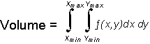
In Surfer, this is computed by first executing a directional integration along the X-axis (across columns) to find cross-sectional areas beneath rows, and then integrating those values along the Y-axis to output absolute cubic volume. This integration methodology is verified in Press, et al., 1988, Section [4.6].
Units
Volumetric cubic values are only mathematically valid if your horizontal (X,Y) and vertical (Z) axes share identical physical units.

|
If a grid uses geographic units (Latitude/Longitude degrees) for X, Y location and linear units (meters or feet) for height, your volume output represents an invalid calculation. |
To normalize a mixed-unit dataset, re-project the grid file into a local planar projection (such as UTM or State Plane) via the Project command before running any volume operations. Alternatively, apply coordinate transformations directly to your raw worksheet data columns via project the X and Y columns before initial grid matrix generation.
Example 1
A grid file configured with uniform X, Y, and Z units in feet yields results in cubic feet (feet)³.
Net Volume = (feet * feet * feet)
Example 2
A grid file configured with uniform X, Y, and Z units in meters yields results in cubic meters (meters)³.
Net Volume = (meter * meter * meter)
See Also
Introduction to Volumes, Areas, Cross Sections