Grid Calculus

Click the Grids | Calculate | Calculus command or the button to access tools to interpret your grid files. Grid calculus can help you define and quantify characteristics in the grid file that might not be obvious by looking at a contour or 3D wireframe of the grid.

The Grids | Calculate | Calculus command creates a new grid file of the generated data. Generated grid files use the same dimensions as the original grid file but might use different ranges of data depending on the type of output.

When a numerical derivative is needed, central difference formulae are used in the calculus computations in Surfer. Because a central difference approach is used, values on both sides of the location for which the derivative is computed are required. This leads to NoData values along the edges of the derivative grids, otherwise known as an edge effect.

Surfer uses "compass-based" grid notation to indicate the neighboring grid nodes used for many of the Grid Calculus operations, as illustrated below:

$image\compass.png$

Using this grid notation, we can write the difference equation approximations for the necessary derivatives at location Z as follows:

$image\img00141.png$

$image\img00142.png$

$image\img00143.png$

$image\img00144.png$

$image\img00145.png$

$image\img00146.png$

$image\img00147.png$

$image\img00148.png$

The Grid Calculus Dialog

Click the Grids | Calculate | Calculus command to open the Grid Calculus dialog.

The Grid Calculus dialog provides four sections of commands to interpret your grid file.

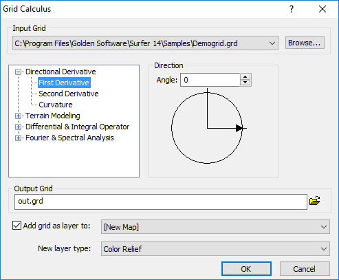
The Grid Calculus dialog is divided into four sections:

Input Grid

Specify the source map layer or grid file in the Input Grid section. Click the current selection and select a map layer from the list. Only map layers created from grid files are included in the Input Grid list. Click Browse to load a grid file with the Open Grid dialog.

Output Grid

Type a file path and file name, including the file type extension, in the Output Grid field, or click the $image\open2.png$ button and specify the path and file name for the grid file in the Save Grid As dialog.

Add New Map or Layer

Check the Add grid as layer to check box to automatically add the created grid to a new or existing map. Select [New Map] in the Add grid as layer to field to create a new map. Click the current selection and select an existing map to add a new layer to the map. Select the layer type by clicking the current selection in the New layer type field and selecting the desired layer type from the list.

Note: If you are saving the grid file in the DEM grid format, clear the Add grid as layer check box and add the map or layer with a Home | New Map or Home | Add to Map | Layer command.

Using Grid Calculus

To create a grid using Grid | Calculus :

Click the Grids | Calculate | Calculus command.
Select the grid map layer or grid file in the Input Grid section.
Expand the calculus type you wish to use by clicking on the next to the type name.
Select a calculus operation (e.g. terrain slope).
If available, set the options for the operation.
Click the button to set the Output Grid path and file name.
Click OK and the new grid file is created.

Grid Calculus and .GSR2 Files

When the input .GRD file for a Grids | Calculate | Calculus command has a defined .GSR2 file with coordinate system information, this information is used for the output .GRD file. The Export Options dialog appears with the option to save the coordinate system information. It is recommended to check the GS Reference (Version 2) file if you intend to use the grid file in Surfer, as the GSR2 retains all of the information needed. The grid has the same coordinate system as the original file, but the .GSR2 is required to define the coordinate system.