Gridding Method Comparison

It is recommended that you try each of the different gridding methods, accepting the defaults, in much the same fashion as you have seen here. This gives you a way to determine the best gridding method to use with the same data set.

In this example, we will use the Demogrid.dat file located in the Samples folder. Each image shows the contour and post map combination created from the default settings for each of the various gridding methods.







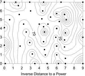
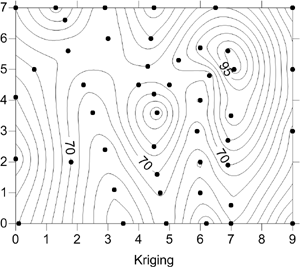
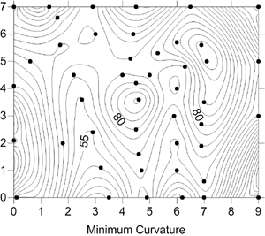
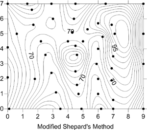
This is a comparison of different gridding methods. For these examples, the sample file, Demogrid.dat, was used. All the defaults for the various methods were accepted. This data set contains 47 data points, irregularly spaced over the extent of the map. The data point locations are displayed as a post map layer.

Achieving Different Results with Different Gridding Methods:

Using the same data set from the Demogrid.dat file and applying different gridding methods produces maps that emphasize different patterns.

Smooth Appearance

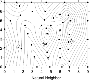
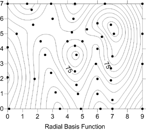
Kriging, Minimum Curvature, Natural Neighbor, and Radial Basis Function all produced acceptable contour maps with smooth appearance.

Bulls Eye Pattern

Inverse Distance to a Power and Modified Shepard's Method both tended to generate "bull's eye" patterns.

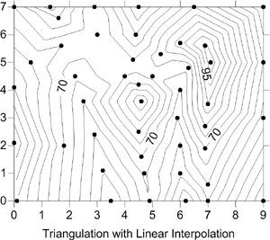
Triangular Facets

With Triangulation with Linear Interpolation, there are too few data points to generate an acceptable map, and this explains the triangular facets apparent on the contour map.

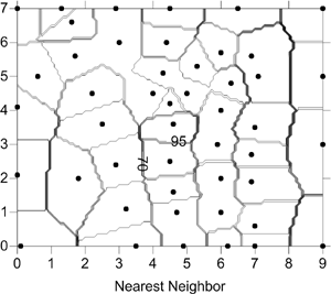
Blocky

Nearest Neighbor shows as a "blocky" map because the data set is not regularly spaced and therefore a poor candidate for this method.

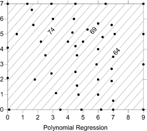
Tilted Plane

Polynomial Regression shows the trend of the surface, represented as a tilted plane.

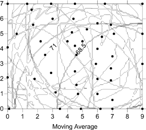
Discontinuities

Due to the small number of data in Demogrid.dat, the Moving Average method is not applicable. The results of using this method with an inadequate data set are shown as discontinuities are created as data are captured and discarded by the moving search neighborhoods.

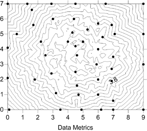
Median Distance

Data Metrics can show many different types of information about the data and about the gridding process, depending on which metric is selected. This example shows the median distance between each grid node and the original 47 data points.

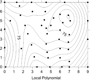
Smooth Local Variation

Local Polynomial models smooth local variation in the data set.