Grid Data - Output (XYZ Data)
The Output page in the Grid Data dialog includes output options for the grid file, including geometry, data limits and transforms, assigning NoData, and generating a report.
|
|
|
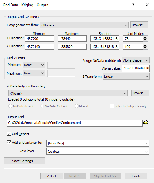
Specify grid file output options in the Output page. |
Output Grid Geometry
The Output Grid Geometry section defines the grid limits and grid density.
Copy Geometry
The Copy geometry from option copies the grid geometry from an existing map layer or grid file. This option is useful if you have many grids that you'd like to all use the same geometry.
To copy the geometry from an existing layer, select the layer in the Copy geometry from list. To copy the geometry from a grid file, click Browse and select the file in the Open Grid dialog. Select <None> to return the Output Grid Geometry options to their default values and to manually edit the grid geometry.
Minimum and Maximum X and Y Coordinate (Grid Limits)
Grid limits are the minimum and maximum X and Y coordinates for the grid. Surfer computes the minimum and maximum X and Y values from the XYZ data file. These values are used as the default minimum and maximum coordinates for the grid.
Grid limits define the X and Y extent of the output grid. The extents of the grid define the extents of contour maps, color relief maps, shaded relief maps, vector maps, 3D wireframes, and 3D surfaces created from grid files. When creating a grid file, you can set the grid limits to the X and Y extents you want to use for your map. Once a grid file is created, you cannot produce a grid-based map larger than the extent of the grid file. If you find you need larger grid limits, you must regrid the data. You can, however, read in a subset of the grid file to produce a map smaller than the extent of the grid file.
When either the X, Y, or Z value is in a date/time format, the date/time values are converted and stored in the grid as numbers.
Spacing and # of Nodes (Grid Density)
Grid density is usually defined by the number of columns and rows in the grid, and is a measure of the number of grid nodes in the grid. The # of Nodes in the X Direction is the number of grid columns, and the # of Nodes in the Y Direction is the number of grid rows. The direction (X Direction or Y Direction) that covers the greater extent (the greater number of data units) is assigned 100 grid nodes by default. The number of grid nodes in the other direction is computed so that the grid nodes Spacing in the two directions are as close to one another as possible.
By defining the grid limits and the number of rows and columns, the Spacing values are automatically determined as the distance in data units between adjacent rows and adjacent columns.
Note on High Density Grid Files
Higher grid densities (smaller Spacing and a larger # of Nodes) increase the smoothness in grid-based maps. However, an increase in the number of grid nodes proportionally increases the gridding time, drawing time, and the grid file size. You can have up to 2,147,483,647 rows and columns in a grid file. It is likely your computer will run out of memory before reaching the maximum grid size. The primary use for the large grid size maximum is to allow grids with extreme aspect ratios to be created.
The larger the density of grid nodes in the grid, the smoother the map that is created from the grid. Contour lines and XY lines defining a wireframe are a series of straight-line segments. More X and Y grid nodes in a grid file result in shorter line segments for contours or wireframe maps. This provides a smoother appearance to contour lines on a contour map or smoother appearing wireframe.
Although highly dense grid files can be created, time and space are practical limits to the number of grid nodes you may want to create in a grid file. The grid density limit is based on the amount of available memory in your computer and the size of the data file used to create the grid. Limited memory, very large data files, very dense grids, or any combination of these factors can greatly increase gridding time. When gridding begins, the status bar provides you with information about the estimated gridding time to complete the task. If gridding time is excessive, click in the plot window to cancel the gridding operation.
Some examples of the amount of memory needed to grid large files:
- A 10,000 x 10,000 grid requires 10000*10000*8 = 763MB.
- A 15,000 x 15,000 grid requires 1.7GB.
- A 20,000 x 20,000 grid requires 3GB.
- A 2,147,483,647 x 2 grid requires 32GB of contiguous RAM (most computers contain a maximum of 16GB RAM stored noncontiguously)
You can also increase or decrease the grid density by using the Grid | Spline Smooth, Grid | Extract, or Grids | Resize | Mosaic commands.
Output Grid Geometry Example
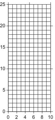
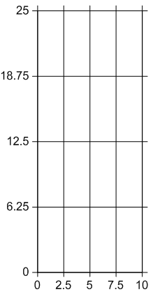
Consider these examples. The data range from 0 to 25 in the Y dimension and 0 to 10 in the X dimension. The two examples use different numbers of grid nodes, or grid spacing, during gridding.
|
|
|
Two different Grid Line Geometry examples are shown here. These are based on the same data file. The coordinates range from zero to 10 in the X direction and zero to 25 in the Y dimension. |
|
In the example on the left above, the grid Spacing is set approximately equal in the X and Y dimensions (one unit each). This results in a different number of grid nodes in the X and Y dimensions. In the example on the right above, the same # of Nodes are specified in the two dimensions. This results in an unequal spacing in data units in the two dimensions.
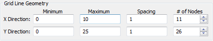
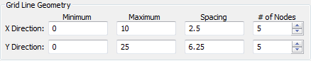
The Output Grid Geometry information specified in the Grid Data dialog for each of the examples is displayed below.
|
|
|
This shows the Output Grid Geometry information for the 11 by 26 grid. The grid node spacing values are set to one, resulting in a different number of grid nodes in the X and Y dimensions. |
|
|
|
This shows the Output Grid Geometry information for the 5 by 5 grid. The number of nodes is equal, resulting in different spacing in the X and Y dimensions. |
Grid Z Limits
In some cases, the gridding interpolation and extrapolation can result in undesired values, for example negative numbers in cases where negative values are physically impossible. The Grid Z Limits options clamp the grid output to specific minimum and maximum values.
The Grid Z Limits are applied after the interpolation operation. After the grid interpolation is performed, Surfer locates any grid values less than the Minimum and replaces them with the Data min or Custom value. Surfer locates any grid values greater than the Maximum and replaces them with the Data max or Custom value.
To clamp the output to a specific minimum value, click the current selection next to Minimum, and select None, Data min, or Custom from the list. If Data min is selected, the data minimum will be displayed in the field to the right of the Minimum list. Select Custom and type a value in the input box to use a user-defined Minimum.
To clamp the output to a specific maximum value, click the current selection next to Maximum, and select None, Data max, or Custom from the list. If Data max is selected, the data maximum will be displayed in the field to the right of the Maximum list. Select Custom and type a value in the input box to use a user-defined Maximum.
Assign NoData outside of
2D Convex Hull
Select 2D Convex hull from the Assign NoData outside of list to assign the NoData value to the grid nodes outside the 2D convex hull of the data. The 2D convex hull of a data set is the smallest convex polygon containing all the data. The 2D convex hull can be thought of as a rubber band that encompasses all data points. The rubber band only touches the outside points. Areas inside the 2Dconvex hull without data are still gridded.
If 2D Convex hull is selected from the Assign NoData outside of list, the Grid Data dialog displays the Inflate convex hull by box. Enter a value to expand or contract the 2D convex hull. When set to zero, the boundary connects the outside data points exactly. When set to a positive value, the area assigned the NoData value is moved outside the 2D convex hull boundary by the number of map units specified. When set to a negative value, the area assigned the NoData value is moved inside the 2D convex hull boundary by the number of map units specified. Values are in horizontal (X) map units. If the value is set to a large positive value, the grid values may extend all the way to the minimum and maximum X and Y limits of the grid, essentially overriding the Assign NoData outside 2D convex hull of data option. If the value is set to a large negative value, the entire grid may be assigned the NoData value, resulting in no grid file being created.
2D Convex Hull Example
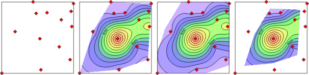
This example, with a data set such as the points on the left below, checking the Assign NoData outside 2D convex hull of data option will leave the outer edges of the map blank due to the NoData values in these areas. The three contour maps display the resulting grid file when the Inflate convex hull by option is set to 0, inflated by 1.5, and deflated by -1.5. Contours always extend to the same minimum and maximum X and Y coordinates. Contour lines align in all three situations. The only difference is how far the contours extend from the 2D convex hull.
|
|
|
This data has an area near the top left corner with no data. When the Assign NoData outside 2D convex hull of data option is selected, no contours appear in this area. Setting the Inflate convex hull by value to a positive value (3rd image) creates a buffer around the outside of the data points. Setting the Inflate convex hull by value to a negative value (last image) brings the contours inside the 2D convex hull of data. |
2D Alpha Shape
Select 2D Alpha shape from the Assign NoData outside of list to assign the NoData value to the grid nodes outside the alpha value of the data. Select 2D Alpha shape instead of 2D Convex hull to have a tighter boundary, especially if a boundary could form concave areas. If 2D Alpha shape is selected from the Assign NoData outside of list, the Grid Data dialog displays the Alpha value box. Enter a value to define the radius of the circles that are created by the edges of the triangulation of the points. Larger alpha values create a more convex boundary and smaller alpha numbers create a tighter, concave boundary. If too low or too high of an alpha value was entered, a message will appear stating that the grid could not be assigned NoData because of the alpha value. For more information on alpha shapes or to determine an appropriate alpha value, see the Alpha Shape help topic.
Z Transform
The Z Transform option changes how the Z values are gridded. Available options are Linear; Log, save as log; and Log, save as linear. To change the Z Transform option, click on the existing option and select the desired option from the list.
Linear uses the Z values in the worksheet for gridding. No transformation is applied to the Z values. The Linear method is a good option for data that gradually increases over space. This is the default Z Transform.
Both Log options use take the log (base 10) of the Z values before gridding. The log (base 10) of the Z value is then used for gridding. The Log, save as log takes the log (base 10) of the Z values and uses the log value for gridding. The grid is then saved with the log (base 10) values. The Log, save as linear takes the log (base 10) of the Z values and uses the log value for gridding. The grid is then converted back to the linear Z values by taking the antilog of the gridded results. When Log, save as log or Log, save as linear is selected, at least three data points must be positive Z values. Negative values are ignored for gridding. Both Log methods are good options when the data changes very quickly over a small area or when very high and very low values occur very closely to each other. This can be common with concentration values in ground water or geochemical data.
|
|
|
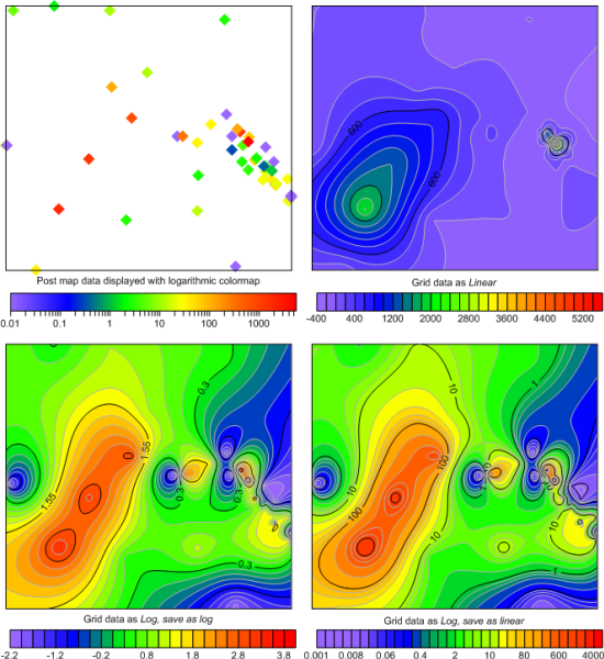
The images above display the difference in gridding the posted data with linear (top right) and log (bottom contours). The log contours on bottom show the difference in Z values between the grid when Log, save as log (bottom left) and Log, save as linear (bottom right) are selected. |
NoData 2D Polygon Boundary
Specify the region or regions to be assigned the NoData value and whether or not to use only selected objects in the NoData 2D Polygon Boundary section. Select either a map layer or vector file in the NoData 2D Polygon Boundary section:
-
Click the current selection and select a base layer from the list. Only base layers that contain at least one eligible polygon or polyline will be included in the list. The base layer must use the same source coordinate system as the grid.
-
Click Browse to load a vector file with the Open dialog. The file must use the same coordinate system as the grid.
The number of polygons and vertices is displayed below the NoData 2D polygon boundary once a file or map layer has been selected. If the boundaries have blanking flags or BLN_Flag attributes, the total number of inside and outside flags is displayed.
Note that all boundaries are treated as 2D polygon boundaries when assigning NoData meaning that only the XY coordinates are used when determining which grid nodes will be assigned the NoData value. For 3D grids, this means that the same XY boundary will be used to assign NoData at all Z levels.
Polyline Boundaries
2D and 3D polylines can be used for NoData polygon boundaries. The polylines in the base layer or vector file will be treated as polygons and 3D polylines treated as 3D polygons while assigning NoData values. The Assign NoData command is not recommended with open polylines as unexpected results may occur. Before clicking Grids | Edit | Assign NoData, consider converting the object to another type better suited to the operation you wish to perform with one of the Change To commands, and edit features with the Reshape command.
If the layer you wish to use contains both polygons and polylines, but you only wish to use some or all of the polygons, select the objects you wish to use before clicking Grids | Edit | Assign NoData and select the Selected objects only option. If the file you wish to use contains both polylines and polygons, first load the file as a base layer, and then use the Assign NoData command with the Selected objects only option.
Inside, Outside, or Mixed
Select Inside to assign the NoData value to the region inside the NoData polygon/3D polygon boundary or boundaries. Select Outside to assign the NoData value to the region outside the NoData polygon/3D polygon boundary or boundaries. Select Mixed to use the blanking flag or BLN_Flag attribute values from the file or layer. The Mixed option is only available when the layer or file contains both blanking flags or BLN_Flag attributes: assign NoData inside (1) and assign NoData outside (0). If all blanking flags or BLN_Flag attributes are the same, the NoData Inside or NoData Outside option is selected automatically, and the Mixed option is not available.
Selected Objects Only
Select the Selected objects only option to use only the selected objects in the base layer to assign NoData values to the grid. When the Selected objects only box is checked, the Loaded polygonsandvertices values are updated. Select a base layer in the NoData 2D Polygon Boundary field to use the Selected objects only option. The Selected objects only option is not available when the NoData 2D Polygon Boundary is a vector file. The polygon or polygons must be selected before clicking the Grids | Edit | Assign NoData command.
Supported Vector Formats
The following file formats can be used to assign NoData values to a grid based on a polygon boundary:
Output Grid
Choose a path and file name for the grid file in the Output Grid group. You can type a path and file name, or click the  button to browse to a new path and enter a file name in the Save Grid As dialog.
Click the coordinate system icon (globe  ) next to the output file path to view or assign a coordinate system to the resulting grid file. If the input data lacks a referenced coordinate system, the icon will display a question mark (
 ); click it to assign the data's native coordinate system. Please note this tool should only be used to assign the input data's existing coordinate system, not to convert or project the data into a new system.
Grid Report
Check the box next to the Grid Report option to create a gridding report that includes all the gridding parameters used to generate a grid. This report also includes statistics about the grid. You can also access the grid statistics by creating a grid information report. Create a grid information report in the Grid Editor by clicking the Grid Editor | Options | Grid Info command or by clicking the Grids | Info | Grid Info command from any document window.
Add New Map or Layer
Check the Add grid as layer to check box to automatically add the created grid to a new or existing map. Select [New Map] in the Add grid as layer to field to create a new map. Click the current selection and select an existing map to add a new layer to the map. Select the layer type by clicking the current selection in the New layer type field and selecting the desired layer type from the list.
Save Settings
Click Save Settings to save the current Grid Data dialog settings from all dialog pages (Select Data, Variogram (if applicable), Options, Cross Validation, and Output) to a Grid Data Settings file. Grid Data Settings files can be loaded on the Select Data page when creating grids.
What's Next?
Click Finish to create the grid file, or click Back to return to previous dialog pages.