Map Types

Several different map types can be created, modified, and displayed with Surfer. These map types include base, contour, post, classed post, 3D surface, 3D wireframe, color relief, grid values, drillhole, peaks and depressions, point cloud, watershed, viewshed, 1-grid vector, and 2-grid vector maps. A brief description and example of each map is listed below.

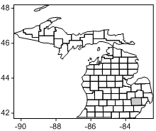
This is a base map of Michigan with county polygons. One of the individual polygons has fill.

Base Map

Base maps display boundaries on a map and can contain polygons, polylines, 3D polygons, 3D polylines, 3D polymesh objects, points, text, images, or metafiles. Base maps can be overlaid with other map layers to provide details such as roads, buildings, streams, city locations, areas of no data, and so on. Base maps can be produced from vector files, images, and data files. Individual base map objects can be edited, moved, reshaped, or deleted. Symbology can be added to a base map to communicate statistical information about the map features. Empty base maps can be created and used for drawing objects on other maps. Raster (image) and vector base maps can be downloaded from online WMS, OSM, WCS and WFS mapping servers.

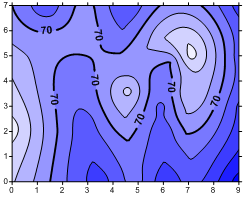
This is a contour map consisting of contour lines representing elevation.

Contour Map

Contour maps are two-dimensional representations of three-dimensional data. Contours define lines of equal Z values across the map extents. The shape of the surface is shown by the contour lines. Contour maps can display the contour lines and colors or patterns between the contour lines. Contours can be linearly or logarithmically spaced, or a custom spacing can be set between each set of lines.

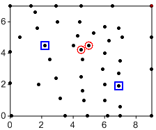
The post map layer has black symbols. The classed post map layer has red circles and blue squares. Only a sample of the data set is displayed in the classed post map.

Post Map

Post maps and classed post maps show data locations on a map. You can customize the symbols and text associated with each data location on the map. Each location can have multiple labels. Classed post maps allow you to specify classes and change symbol properties for each class. Classes can be saved and loaded for future maps.

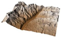
This is a 3D surface map of the Telluride, Colorado USGS SDTS grid file.

3D Surface Map

3D surface maps are color three-dimensional representations of a grid file. The colors, lighting, overlays, and mesh can be altered on a surface. Multiple 3D surface maps can be layered to create a block diagram.

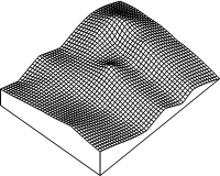
This is a 3D wireframe map with a custom rotation (47° ), tilt (49° ), and field of view (112° ).

3D Wireframe Map

3D wireframe maps are three-dimensional representations of a grid file. Wireframes are created by connecting Z values along lines of constant X and Y.

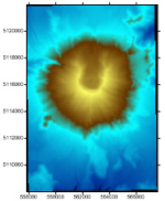
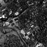
This is a color relief map of the Helens2.grd sample file.

Color Relief Map

Color relief maps are raster images based on grid files. Color relief maps assign colors based on Z values from a grid file. NoData regions on the color relief map are shown as a separate color or as a transparent fill. Pixels can be interpolated to create a smooth image. Hill shading or reflectance shading can be applied to the color relief map to enhance its depth and appearance.

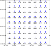
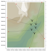
The grid values layer posts symbols, labels, and/or lines along grid rows and columns at a specified density.

Grid Values Map

Grid values maps show symbols labels at grid node locations across the map. The density of the labels and symbols is controlled in the X and Y directions independently. Symbol color can vary by value across a colormap, and symbols and labels can be displayed for only a specific range of values. Grid lines can be added to the map.

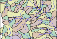
This is a watershed map of a USGS SDTS grid file.

Watershed Map

Watershed maps display the direction that water flows across the grid. The watershed map breaks the grid into drainage basins and streams. Colors can be assigned to the basins and line properties can be associated with the streams. In addition, depressions can be removed by filling the depression.

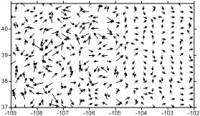
This is a 1-grid vector map of Colorado elevations.

Vector Map

1-grid and 2-grid vector maps display direction and magnitude data using individually oriented arrows. At any grid node on the map, the arrow points in the downhill direction of the steepest descent and the arrow length is proportional to the slope magnitude. Vector maps can be created using information in one grid file (i.e. a numerically computed gradient) or two different grid files (i.e. each grid giving a component of the vectors).

This is a point cloud of the Golden, CO area from USGS Elevation Source Data

Point Cloud Map

Point cloud maps display LAS/LAZ data as points at XY locations. LAS/LAZ data can be combined from multiple files and filtered with various criteria when creating a point cloud map. Color is assigned to the points by elevation, intensity, return number, or classification. Surfer includes commands for modifying, classifying, and exporting points in a point cloud layer. A grid can be created from the point cloud layer. Point cloud layers are displayed in the 3D View as three-dimensional points.

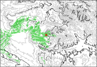
This is a viewshed layer overlaid on a contour map.

Viewshed Layer

Viewshed layers highlight the regions of a map that are visible (or invisible) from a transmitter location. The transmitter, receiver, and obstruction height above the surface can be specified. The viewshed analysis radius and angle can also be specified. Viewsheds can be added to any 2D grid based map. A viewshed can also be added to a 3D surface map that is displayed with no tilt (90 degrees) and in the orthographic view.

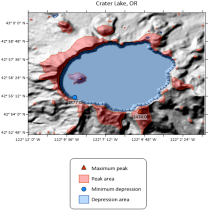
The legend for this peaks and depressions map of the Crater Lake area explains the shaded areas and markings.

Peaks and Depressions Map

Volumes of surface water and ground water are informed by topographic data, Karst topography, and geographic data, which are captured in Surfer grid files and mapped in peaks and depression maps. Boundaries can be drawn around peaks where water flows from and depressions which capture water to create unique areas for statistical analysis.

This is a drillhole layer created using the SampleDrilholeData sample files.

Drillhole Map

A drillhole map can be created from collars, survey, intervals, and point data. The 2D drillhole layer shows the location, deviation, and path of each hole, core, or well. The drillhole map can also be viewed in 3D. Separate symbols can be defined to create a legend of the drillholes by hole id or any other attribute in the data.